To address this challenge, TVM takes a full stack compiler approach. TVM combines code generation and auto-tuning to generate kernels that are comparable to heavily hand-optimized libraries, obtaining state-of-the-art inference performance on hardware platforms including ARM CPUs, Intel CPUs, Mali GPUs, NVIIDA GPUs and AMD GPUs.
In this blog post, we show the workflow of automatic kernel optimization in TVM compiler stack and benchmark results on several hardware platforms.
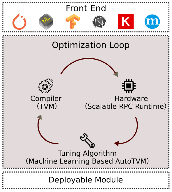
Kernel optimization in TVM is done in an iterative loop fashion. As shown in Figure 1, the automatic kernel optimization takes a neural network (typically in computational graph representation) from frontend frameworks as input, and generates kernels for all operators in this network.
The inner loop uses a scalable RPC runtime, machine learning based tuners and a tensor compiler. In each round of the loop, the tuner picks a batch of promising candidate kernel implementations from a large search space, and profile them on real hardware. Then the tuner gets the profiling results. These profiling results are used as training data to fit a prediction model. After fitting the prediction model, the tuner picks the next promising candidates according to the predictions, and the loop continues. This way, we search for fast kernels iteratively.
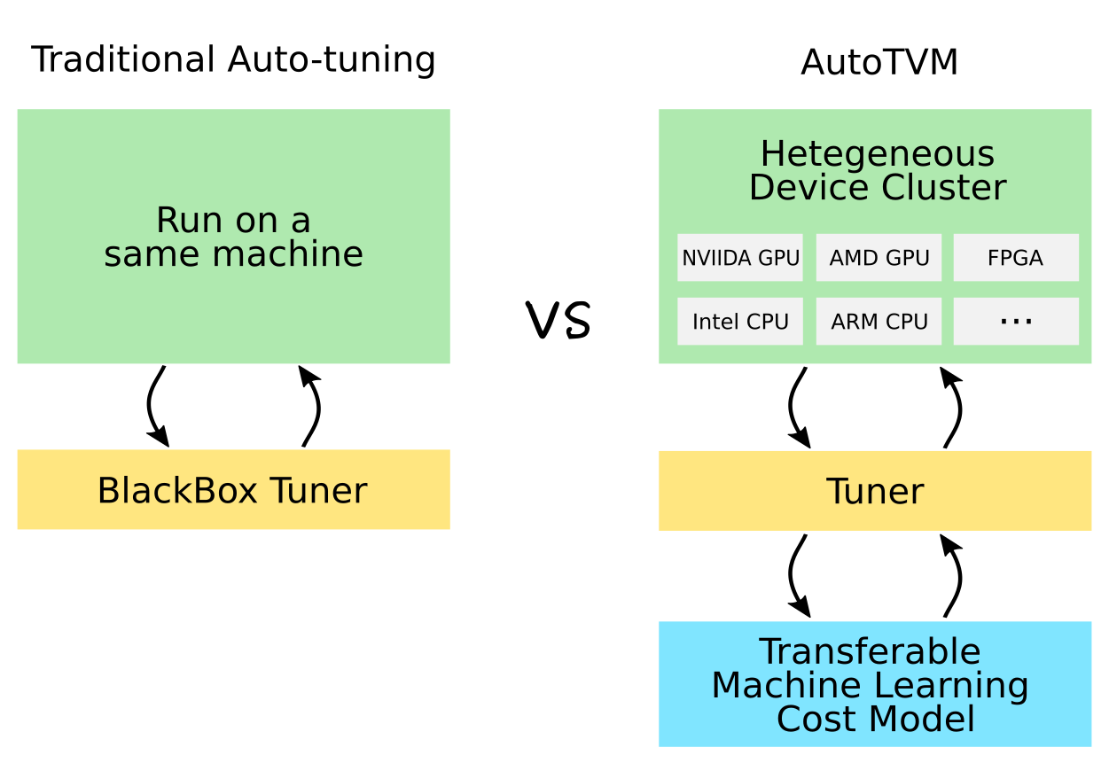
The below figure compares traditional auto-tuning and AutoTVM. The major difference is that AutoTVM is
You can refer to our paper[1] for more details.
For demonstration, we run our optimization for resnet-18 on RK3399, an ARM development board. The detailed instructions are omitted due to the space limit of a blog post. Links to tutorials for ARM CPU, Mali GPU, NVIDIA GPU, AMD GPU are all available at the end of this blog.
First we get a pre-trained model from MXNet model zoo, and extract tuning tasks from it.
from mxnet.gluon.model_zoo.vision import get_model
block = get_model('resnet18_v1', pretrained=True)
net, params = nnvm.frontend.from_mxnet(block)
tasks = autotvm.extract_from_graph(net)
tune_tasks(tasks, **tuning_option)
There are 12 different conv2d layers in resnet-18, so we launch 12 tuning tasks. For each of them, the tuner makes several hundreds of trials and picks the best one. After finishing all tuning tasks, we compile the whole network and generate a single deployable minimal library. One sample output is
Extract tasks...
Tuning...
[Task 1/12] Current/Best: 22.37/ 52.19 GFLOPS | Progress: (544/1000) | 406.59 s Done.
[Task 2/12] Current/Best: 6.51/ 18.77 GFLOPS | Progress: (608/1000) | 325.05 s Done.
[Task 3/12] Current/Best: 4.67/ 24.87 GFLOPS | Progress: (480/1000) | 372.31 s Done.
[Task 4/12] Current/Best: 11.35/ 46.83 GFLOPS | Progress: (736/1000) | 602.39 s Done.
[Task 5/12] Current/Best: 1.01/ 19.80 GFLOPS | Progress: (448/1000) | 262.16 s Done.
[Task 6/12] Current/Best: 2.47/ 23.76 GFLOPS | Progress: (672/1000) | 563.85 s Done.
[Task 7/12] Current/Best: 14.57/ 33.97 GFLOPS | Progress: (544/1000) | 465.15 s Done.
[Task 8/12] Current/Best: 1.13/ 17.65 GFLOPS | Progress: (576/1000) | 365.08 s Done.
[Task 9/12] Current/Best: 14.45/ 22.66 GFLOPS | Progress: (928/1000) | 724.25 s Done.
[Task 10/12] Current/Best: 3.22/ 15.36 GFLOPS | Progress: (864/1000) | 564.27 s Done.
[Task 11/12] Current/Best: 11.03/ 32.23 GFLOPS | Progress: (736/1000) | 635.15 s Done.
[Task 12/12] Current/Best: 8.00/ 21.65 GFLOPS | Progress: (1000/1000) | 1111.81 s Done.
Compile...
Upload...
Evaluate inference time cost...
Mean inference time (std dev): 162.59 ms (0.06 ms)
The tuning is especially helpful and worth a try if your model has some strange shapes or your hardware is customized, as hand-optimized static libraries cannot consider all situations.
We pre-tuned some popular networks on our device cluster and released the following benchmark. Instructions for reproduction are at the end of this blog.
Comprehensively benchmarking TVM is easy since we have a unified runtime interface. However maintaining complete, up-to-date, and correct comparisons against all other platforms is not feasible without expert assistance from the developers of many other projects. So we put all our numbers in a table, and then provide an incomplete comparison with some other libraries.
We validate the effectiveness of our automatic optimization stack by comparing with heavily optimized traditional libraries on each platform.
We tested popular image classification networks on ImageNet (3x224x224) dataset with batch size = 1 and data type = float32. The reported numbers are time costs per image in milliseconds.
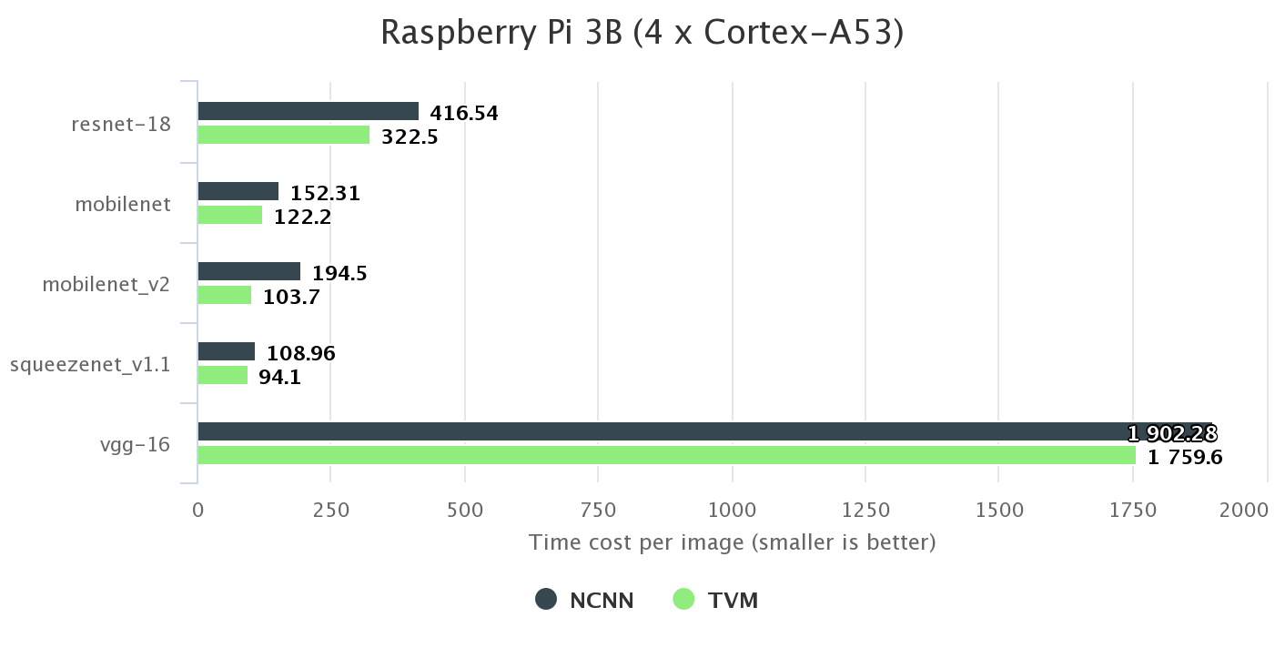
We choose NCNN, a widely used, hand-optimized kernel library as baseline. It makes extensive use of NEON assembly instructions. For example, the code base contains 13k lines of code for only 3x3 convolution layers. We reference the benchmark numbers in their project repository. As shown in the figure below, TVM outperforms it for all networks on Rasbperry Pi 3B.
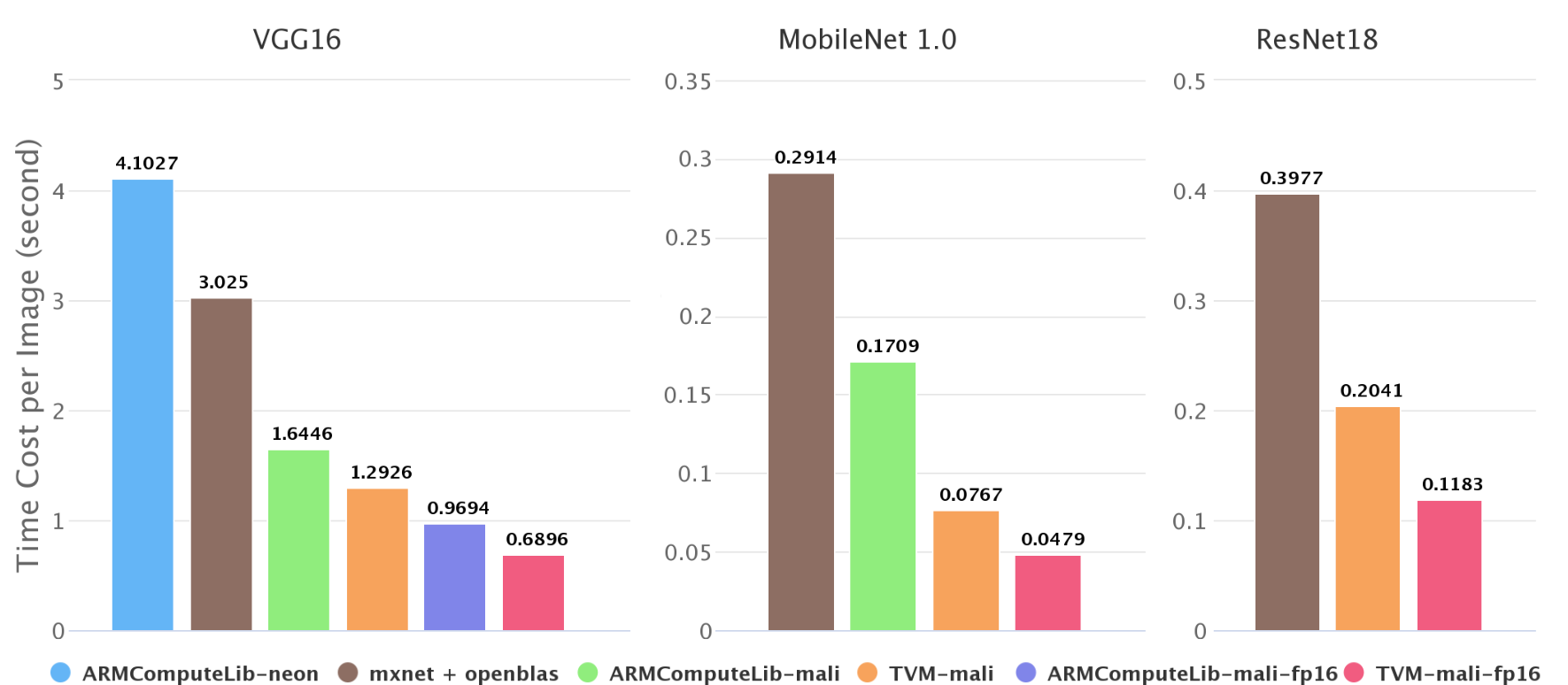
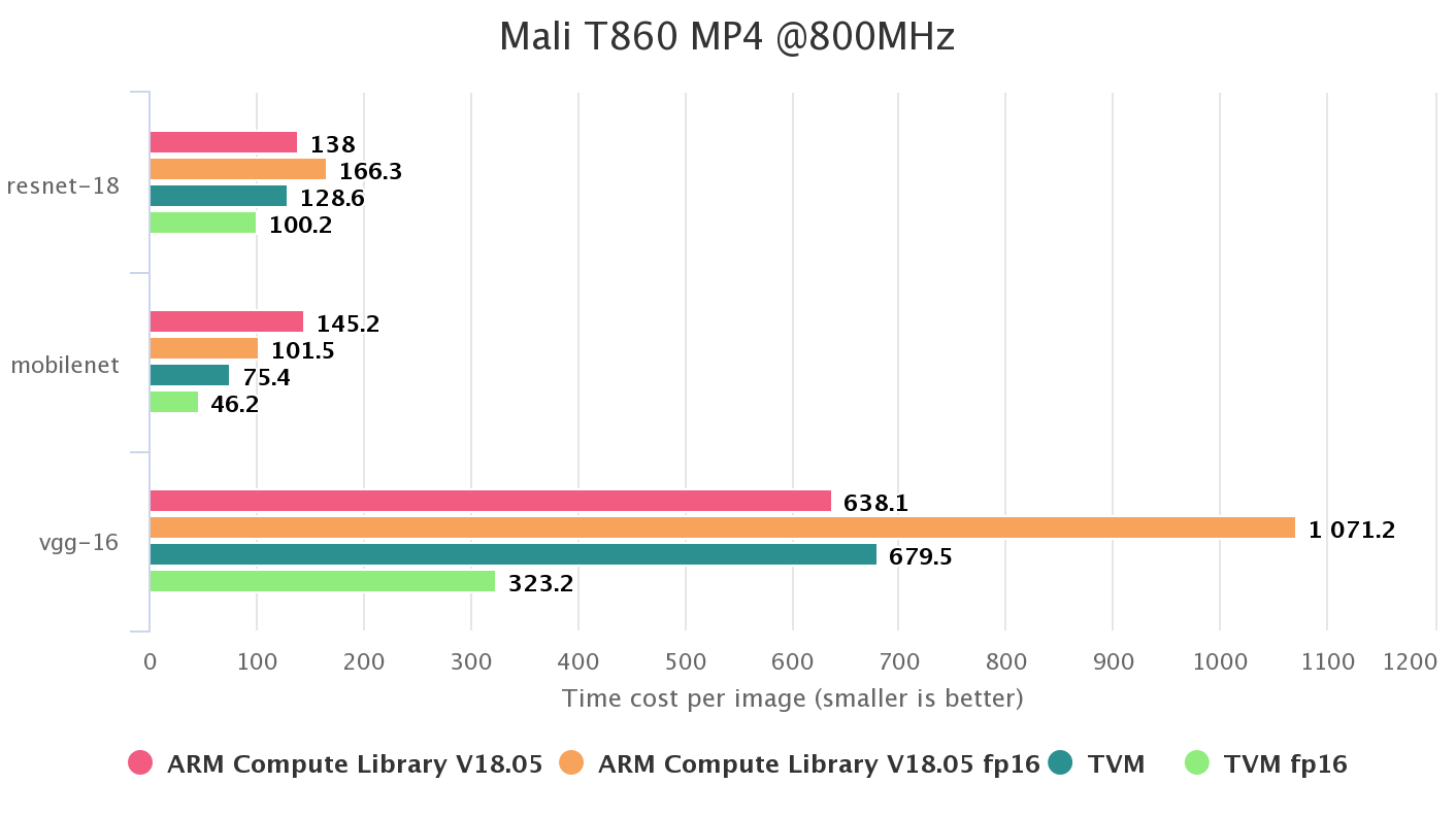
ARM Compute Library is a vendor provided library that supports Mali GPU (OpenCL) well, so it is selected as baseline. According to the results, TVM outperforms ARMComputeLib on most networks for single precision (fp32) and achieves the best performance on this board by using half precision (fp16). TVM shows better scalibility when shifting from fp32 to fp16, while ARMComuteLib fails to optimize for fp16 (using fp16 is even slower in some cases).
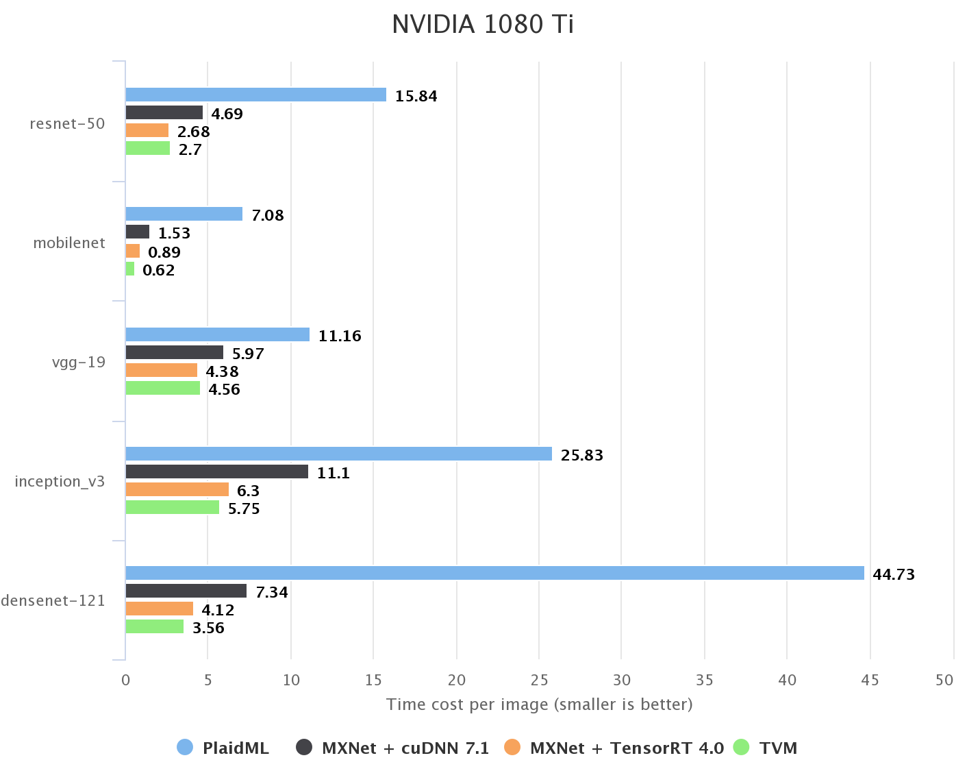
On NVIDIA GPU, CuDNN and TensorRT are two vendor-provided libraries for training and inference respectively. Since we focus on inference, we run our benchmark in the unbatched setting. Another tensor compiler PlaidML is also reported as baseline as there is a previous benchmark of it compared against a pre-AutoTVM version of TVM. We reference its benchmark results from PlaidBench. According to the results below, TVM achieves parity with TensorRT performance.
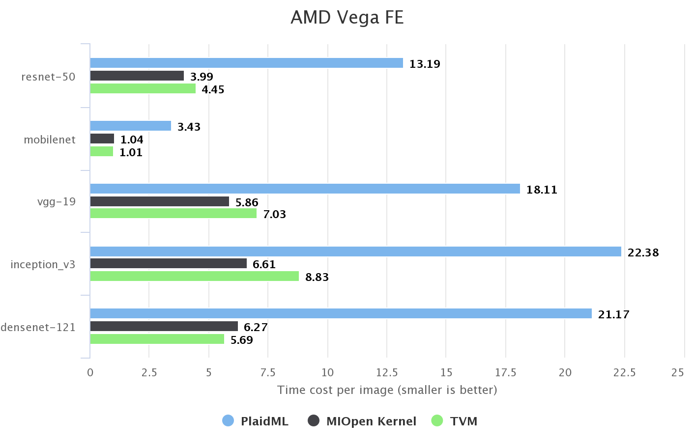
We also take a quick look at a AMD GPU. TVM supports OpenCL and ROCm backend. We found ROCm is better since it is more specialized for AMD GPUs. MIOpen is a vendor provided kernel library. TVM’s graph runtime can call MIOpen’s kernel implementations directly, so we report the baseline performance by using this integration.
We didn’t do any specific optimization for AMD GPU. All computation definition and schedule code for NVIDIA GPU is directly reused. As a result, TVM is a little bit slower then MIOpen in most cases. We believe there is still room for improvement.
We tested the following networks on ImageNet (3x224x224) dataset with batch size = 1 and data type = float32. The reported numbers are time costs per image in millisecond.
densenet121 | inception v3 | mobilenet | mobilenet v2 | resnet18 | resnet50 | squeezenet v1.0 | squeezenet v1.1 | vgg16 | vgg19 | |
---|---|---|---|---|---|---|---|---|---|---|
ARM CPU | ||||||||||
Huawei P20 Pro | 181.4 | 439.9 | 41.1 | 34.5 | 76.5 | 208.2 | 51.8 | 25.7 | 480.6 | 627.0 |
Google Pixel2 | 162.2 | 433.5 | 39.5 | 30.1 | 61.1 | 181.3 | 47.3 | 23.2 | 391.1 | 487.7 |
Firefly RK3399 | 335.9 | 1285.9 | 78.6 | 66.7 | 161.2 | 403.8 | 94.6 | 48.5 | 902.9 | 1090.1 |
Raspberry Pi 3B | 609.5 | 2070.4 | 122.2 | 103.7 | 322.5 | 725.8 | 185.1 | 94.1 | 1759.6 | 2118.6 |
Xilinx PYNQ | 2888.3 | 9709.1 | 723.5 | 514.3 | 1234.6 | 3580.5 | 909.9 | 477.3 | -(Note 1) | - |
Mali GPU | ||||||||||
Mali-T860 MP4 | 410.9 | 783.1 | 75.4 | 70.8 | 128.6 | 352.9 | 106.2 | 58.0 | 679.5 | 805.3 |
Mali-T860 MP4 (fp16) | 410.9 | 783.1 | 75.4 | 70.8 | 128.6 | 352.9 | 106.2 | 58.0 | 679.5 | 805.3 |
NVIDIA GPU | ||||||||||
GTX 1080 Ti | 3.6 | 5.8 | 0.6 | - (Note 2) | - | 2.7 | - | - | 4.0 | 4.6 |
GTX TITAN X | 5.8 | 9.7 | 1.0 | - | - | 4.3 | - | - | 6.4 | 7.5 |
Tegra X2 | 26.4 | 45.4 | 5.1 | - | - | 25.8 | - | - | 57.2 | 67.6 |
AMD GPU | ||||||||||
AMD Vega FE | 5.7 | 8.8 | 1.0 | - | - | 4.5 | - | - | 5.9 | 7.0 |
With an expressive code generator and an efficient search algorithm, we are able to generate kernels that are comparable to heavily hand-optimized ones. Since programmer time is expensive and machine time is getting cheaper, we believe automatic optimization with real hardware and data in the loop will be the standard workflow for inference deployment. TVM just provides such a solution.
[1] benchmark: https://github.com/dmlc/tvm/tree/master/apps/benchmark
[2] Tutorial about tuning for ARM CPU: https://docs.tvm.ai/tutorials/autotvm/tune_nnvm_arm.html
[3] Tutorial about tuning for Mobile GPU: https://docs.tvm.ai/tutorials/autotvm/tune_nnvm_mobile_gpu.html
[4] Tutorial about tuning for NVIDIA/AMD GPU: https://docs.tvm.ai/tutorials/autotvm/tune_nnvm_cuda.html
[5] Paper about AutoTVM: Learning to Optimize Tensor Program
[6] Paper about Intel CPU (by AWS contributors) : Optimizing CNN Model Inference on CPUs
TVM addresses the difficulty of deploying for different hardwares by introducing an unified IR stack, with which the optimization for different hardwares can be done easily. In this post, we show how we use TVM/NNVM to generate efficient kernels for ARM Mali GPU and do end-to-end compilation. In our test on Mali-T860 MP4, compared with Arm Compute Library, our method is 1.4x faster on VGG-16 and 2.2x faster on MobileNet. Both graph-level and operator-level optimization contribute to this speed up.
We will use Firefly-RK3399 with Mali-T860 MP4 as our test environment, so we mainly focus on Mali T8xx below.
Figure 1 is an overview of the Mali Architecture on T860 and T880. The GPUs are scalable up to 16 coherent shader cores. Inside each shader core, there are 2 or 3 arithmetic pipelines, 1 load/store pipeline and 1 texture pipeline (so-called TriPipe). The ALU in each arithmetic pipeline has four 128-bit vector units and one scalar units.
We use OpenCL for GPU computing. When mapping to OpenCL model, each shader core executes one or several work groups. Each shader core supports up to 384 concurrently executing threads. Each work item in OpenCL typically maps to a single thread on a Mali GPU. The Mali GPUs use a VLIW (Very Long Instruction Word) architecture. Each instruction word contains multiple operations. The Mali GPUs also use SIMD, so that most arithmetic instructions operate on multiple data elements simultaneously. [1]
Here are some differences that we should concern when writing OpenCL code for Mali GPUs, compared with writing for NVIDIA’s GPUs.
warp size
is 1, so that branch divergence is not a major problem.The convolution layer is the core of most deep neural networks and takes most of the computation time. So we take the convolution layer as example to demonstrate how common optimization techniques like packing, tiling, unrolling and vectorization are applied in TVM.
A well-known algorithm for convolution layer is im2col, which converts the little 3D input cubes to columns of a matrix and perform a GEMM. The advantage of this method is easy utilization of highly optimized BLAS library. However, the memory redundancy (9x memory for 3x3 kernel) is awful.
Instead, we adopt a method to calculate the convolution, and apply the optimization techniques step by step. A convolution layer in VGG-16 is used as tuning case, whose configuration is listed below. We assume the batch size is 1 for inference.
Input Shape | Output Shape | Kernel Size | Stride | Padding |
---|---|---|---|---|
56x56x256 | 56x56x256 | 3x3 | (1, 1) | (1, 1) |
As a baseline, we also list the performance of this layer in Arm Compute Library.
Kernel | Cost (second) | GFLOPS |
---|---|---|
GEMM method in ARMComputeLib | 0.1821 | 20.3111 |
Tiling and packing are two methods intended for better memory access. Tiling separates the whole computation into small blocks for better datareuse. Packing re-layouts the input matrices according to the tiling so that we can access the memory sequentially, which reduces cache miss rate.
We do tiling on the width dimension of the input image and CO dimension
of the filter matrix. This is described by tvm.compute
.
# set tiling factor
VH = 1
VW = VC = 4
# get input shape
_, CI, IH, IW = data.shape
CO, CI, KH, KW = kernel.shape
TH = IH + 2 * H_PAD
TW = IW + 2 * W_PAD
# calc output shape
OH = (IH + 2*H_PAD - KH) // H_STR + 1
OW = (IW + 2*W_PAD - KW) // W_STR + 1
# data shape after packing
dvshape = (N, TH // (VH*H_STRIDE), TW // (VW*W_STRIDE), CI, VH*H_STRIDE+HCAT, VW*W_STRIDE+WCAT)
# kernel shape after packing
kvshape = (CO // VC, CI, KH, KW, VC)
ovshape = (N, CO // VC, OH // VH, OW // VW, VH, VW, VC)
oshape = (N, CO, OH, OW)
# define packing
data_vec = tvm.compute(dvshape, lambda n, h, w, ci, vh, vw:
data_pad[n][ci][h*VH*H_STRIDE+vh][w*VW*W_STRIDE+vw], name='data_vec')
kernel_vec = tvm.compute(kvshape, lambda co, ci, kh, kw, vc:
kernel[co*VC+vc][ci][kh][kw], name='kernel_vec')
# define convolution
ci = tvm.reduce_axis((0, CI), name='ci')
kh = tvm.reduce_axis((0, KH), name='kh')
kw = tvm.reduce_axis((0, KW), name='kw')
conv = tvm.compute(ovshape, lambda n, co, h, w, vh, vw, vc:
tvm.sum(data_vec[n, h, w, ci, vh*H_STRIDE+kh, vw*W_STRIDE+kw].astype(out_dtype) *
kernel_vec[co, ci, kh, kw, vc].astype(out_dtype),
axis=[ci, kh, kw]), name='conv')
# unpack to correct layout
output = tvm.compute(oshape, lambda n, co, h, w:
conv[n][co//VC][h/VH][w//VW][h%VH][w%VW][co%VC],
name='output_unpack', tag='direct_conv_output')
We can inspect the defined IR by
print(tvm.lower(s, [data, kernel, output], simple_mode=True))
I pick the convolution part here.
produce conv {
for (co, 0, 64) {
for (h, 0, 56) {
for (w, 0, 14) {
for (vw.init, 0, 4) {
for (vc.init, 0, 4) {
conv[((((((((co*56) + h)*14) + w)*4) + vw.init)*4) + vc.init)] = 0.000000f
}
}
for (ci, 0, 256) {
for (kh, 0, 3) {
for (kw, 0, 3) {
for (vw, 0, 4) {
for (vc, 0, 4) {
conv[((((((((co*56) + h)*14) + w)*4) + vw)*4) + vc)] = (conv[((((((((co*56) + h)*14) + w)*4) + vw)*4) + vc)] + (data_vec[(((((((((h*14) + w)*256) + ci)*3) + kh)*6) + kw) + vw)]*kernel_vec[((((((((co*256) + ci)*3) + kh)*3) + kw)*4) + vc)]))
}
}
}
}
}
}
}
}
}
In TVM, we declare the computation at first and then schedule it. This mechanism decouples the algorithm and implementation detail. (This idea is from Halide).
The following schedule simply binds axes to GPU threads, so that our code can run on Mali GPU.
# helper function for binding thread
def tile_and_bind3d(s, tensor, z, y, x, z_factor=2, y_factor=None, x_factor=None):
""" tile and bind 3d """
y_factor = y_factor or z_factor
x_factor = x_factor or y_factor
zo, zi = s[tensor].split(z, z_factor)
yo, yi = s[tensor].split(y, y_factor)
xo, xi = s[tensor].split(x, x_factor)
s[tensor].bind(zo, tvm.thread_axis("blockIdx.z"))
s[tensor].bind(zi, tvm.thread_axis("threadIdx.z"))
s[tensor].bind(yo, tvm.thread_axis("blockIdx.y"))
s[tensor].bind(yi, tvm.thread_axis("threadIdx.y"))
s[tensor].bind(xo, tvm.thread_axis("blockIdx.x"))
s[tensor].bind(xi, tvm.thread_axis("threadIdx.x"))
# set tunable parameter
num_thread = 8
# schedule data packing
_, h, w, ci, vh, vw = s[data_vec].op.axis
tile_and_bind3d(s, data_vec, h, w, ci, 1)
# schedule kernel packing
co, ci, kh, kw, vc = s[kernel_vec].op.axis
tile_and_bind(s, kernel_vec, co, ci, 1)
# schedule conv
_, c, h, w, vh, vw, vc = s[conv].op.axis
kc, kh, kw = s[conv].op.reduce_axis
s[conv].reorder(_, c, h, w, vh, kc, kh, kw, vw, vc)
tile_and_bind3d(s, conv, c, h, w, num_thread, 1, 1)
_, co, oh, ow = s[output].op.axis
tile_and_bind3d(s, output, co, oh, ow, num_thread, 1, 1)
With this schedule, our code can run now, but the performance is terrible.
Kernel | Cost (second) | GFLOPS | speedup |
---|---|---|---|
GEMM method in ARMComputeLib | 0.1821 | 20.3111 | 1x |
Kernel 1: simple bind | 5.6154 | 0.6588 | 0.03x |
Loop unrolling can reduce the instructions for loop control, reduce
branch penalties and hide latency in reading memory.
In TVM, this can be done easily by calling s.unroll(axis)
# set tunable parameter
num_thread = 8
# schedule data packing
_, h, w, ci, vh, vw = s[data_vec].op.axis
tile_and_bind3d(s, data_vec, h, w, ci, 1)
"""!! ADD UNROLL HERE !!"""
s[data_vec].unroll(vw)
# schedule kernel packing
co, ci, kh, kw, vc = s[kernel_vec].op.axis
tile_and_bind(s, kernel_vec, co, ci, 1)
"""!! ADD UNROLL HERE !!"""
s[kernel_vec].unroll(kh)
s[kernel_vec].unroll(kw)
s[kernel_vec].unroll(vc)
# schedule conv
_, c, h, w, vh, vw, vc = s[conv].op.axis
kc, kh, kw = s[conv].op.reduce_axis
s[conv].reorder(_, c, h, w, vh, kc, kh, kw, vw, vc)
tile_and_bind3d(s, conv, c, h, w, num_thread, 1, 1)
"""!! ADD UNROLL HERE !!"""
s[conv].unroll(kh)
s[conv].unroll(kw)
s[conv].unroll(vw)
s[conv].unroll(vc)
_, co, oh, ow = s[output].op.axis
tile_and_bind3d(s, output, co, oh, ow, num_thread, 1, 1)
Kernel | Cost (second) | GFLOPS | speedup |
---|---|---|---|
GEMM method in ARMComputeLib | 0.1821 | 20.3111 | 1x |
Kernel 1: simple bind | 5.6154 | 0.6588 | 0.03x |
Kernel 2: + unrolling | 0.3707 | 9.9796 | 0.49x |
As mentioned before, we need to do vectorization explictly in order to achieve the best performance on Mali GPU.
# set tunable parameter
num_thread = 8
# schedule data packing
_, h, w, ci, vh, vw = s[data_vec].op.axis
tile_and_bind3d(s, data_vec, h, w, ci, 1)
# unroll
s[data_vec].unroll(vw)
# schedule kernel packing
co, ci, kh, kw, vc = s[kernel_vec].op.axis
tile_and_bind(s, kernel_vec, co, ci, 1)
# unroll
s[kernel_vec].unroll(kh)
s[kernel_vec].unroll(kw)
"""!! VECTORIZE HERE !!"""
s[kernel_vec].vectorize(vc)
# schedule conv
_, c, h, w, vh, vw, vc = s[conv].op.axis
kc, kh, kw = s[conv].op.reduce_axis
s[conv].reorder(_, c, h, w, vh, kc, kh, kw, vw, vc)
tile_and_bind3d(s, conv, c, h, w, num_thread, 1, 1)
# unroll
s[conv].unroll(kh)
s[conv].unroll(kw)
s[conv].unroll(vw)
"""!! VECTORIZE HERE !!"""
s[conv].vectorize(vc)
_, co, oh, ow = s[output].op.axis
tile_and_bind3d(s, output, co, oh, ow, num_thread, 1, 1)
Kernel | Cost (second) | GFLOPS | speedup |
---|---|---|---|
GEMM method in ARMComputeLib | 0.1821 | 20.3111 | 1x |
Kernel 1: simple bind | 5.6154 | 0.6588 | 0.03x |
Kernel 2: + unrolling | 0.3707 | 9.9796 | 0.49x |
Kernel 3: + vectorization | 0.1304 | 28.3679 | 1.40x |
As for the tunable parameters above, some can be calculated.
For the vectorized dimension VC
, we should fill the 128-bit register,
so it can be set as 128/32=4 for float32 and 128/16=8 for float16.
But more often we cannot determine the optimal value, due to the complicated runtime. We use grid search in TVM. It can be done extremely effective since we write python code in TVM’s high-level IR rather than direct OpenCL code.
We can view the generated OpenCL code by
print(func.imported_modules[0].get_source())
The OpenCL code is too long to be pasted here, and it is hard to read due to heavy unrolling. If interested, you can view it here.
In this section, we compare the comprehensive performance between different backends on some popular deep neural networks. Our test environment is
Firefly-RK3399 4G
CPU: dual-core Cortex-A72 + quad-core Cortex-A53
GPU: Mali-T860MP4
Arm Compute Library : v17.12
MXNet: v1.0.1
Openblas: v0.2.18
We use NNVM and TVM to do end-to-end compilation.
As shown in Figure 2, we test the inference speed on ImageNet. On Firefly-RK3399, Mali GPU can be 2x ~ 4x faster than 6-core big.LITTLE CPU. Our end-to-end pipeline is 1.4x ~ 2.2x faster than Arm Compute Library. We try both GEMM and direct method of convolution layer in Arm Compute Library, GEMM method is always faster than direct method in these test cases, so we only plot the result of GEMM method.
Some results, like resnet18 on Arm Compute Library, are missing in the Figure 2. It is because the graph runtime of Arm Compute Library does not support skip connection currently and has a poor neon implementation of depthwise convolution. This also reflects the advantage of NNVM software stack.
Precision in deep neural networks is not very important, especially for the inference on mobile devices. Using low-precision arithmetic can make the inference much faster. We also test the half-precision floating number on Mali GPU.
model | backend | Time Cost per Image (second) | speed up to FP32 |
---|---|---|---|
vgg16 | ACM-mali | 0.9694 | 1.69 |
vgg16 | TVM-mali | 0.6896 | 1.87x |
MobileNet 1.0 | TVM-mali | 0.0479 | 1.60x |
ResNet18 | TVM-mali | 0.1183 | 1.73x |
In theory, FP16 can both double peak compute and halve memory consumption, so that doubling the speed. But it needs good input shape for longer vectorization and fine-tuning some parameters.
We should admit that there is still some room for improvement, mainly at the graph level, such as model compression and weight prelayout. Further improvement in NNVM will try to solve these problems.
Lianmin Zheng is an undergraduate student at SJTU Apex lab. He is interested in machine learning and building computer system.
The author has many thanks to Tianqi Chen for his helpful advice and Yizhi Liu for his earlier work.